Likert Scale Analysis
Recently, I worked with researchers at Deaconess Hospital and the University of Southern Indiana. I consulted on a project to analyze Likert data and discovered the long standing controversy on the topic, which was intriguing. Here, I share a little background on Likert data, considerations about the analysis, and basic R code to perform an analysis. In the future, I’ll make available a workflow for to analyze Likert data, and develop a RShiny app to analyze and visualize the results for a standard survey.
knitr::opts_chunk$set(error = TRUE, tidy = TRUE)
wd <- "/Users/jdstallings/Google Drive/Blog/dataindeed/content/post"  # dirname(rstudioapi::getActiveDocumentContext()$path) # sets working directory to where ever you put this document
setwd(wd)

.cran_packages <- c("ggplot2", "sjPlot", "sjmisc", "gridExtra", "cowplot", "grid",
    "tables", "knitr", "pander", "tables", "knitcitations", "png", "downloader",
    "plyr", "data.table", "dplyr", "tidyr", "foreign", "coin", "car", "easyGgplot2",
    "likert", "readxl", "FSA", "plotly", "lattice", "rcompanion", "readr", "mvoutlier",
    "mvnormtest", "HH")  # packages used in this Rmarkdown document

sapply(.cran_packages, require, character.only = TRUE)
Introduction
In 1932, Rensis Likert (pronounced ‘Lik-ert’) developed Likert items to measure respondents’ attitudes to a particular question or statement. For example, the Likert item is typically composed of a statement and series of responses:

Example Likert Item from “A Technique for the Measurement of Attitudes (1932) Archives of Psychology. Volume 22, pp 5-55.”
The Likert responses are typically considered as ordered categorical (i.e., ordinal) data, because they convey size, order, rank or sequence. Responses typically range from positive to negative conceptually, and often there is no actual measurable distance between the responses. We can not assume that a respondent perceives the value between Strongly Approve (1) and Approve (2) to equal the value between Approve (2) and Undecided (3), despite the distance on the scale being the same.
Responses could also use seven or nine answers for more granularity, or only four (or other even number) to avoid neutral or undecided answers, forcing the respondent to select a positive or negative response. Likert responses are not continuous (i.e., there are no actual decimal points in Likert responses), and they are constrained at their ends (i.e., 1-5 is the range in the figure above; there are no responses below the value of 1 or above the value of 5).
The Controversy
In 1946, S.S. Stevens addressed the classification of scales of measurement. Stevens exquisitely described the theory of nominal, ordinal, interval and ratio data, their empirical operations, mathematical group structure and permissible statistics. The table below summarizes his key discussion points:
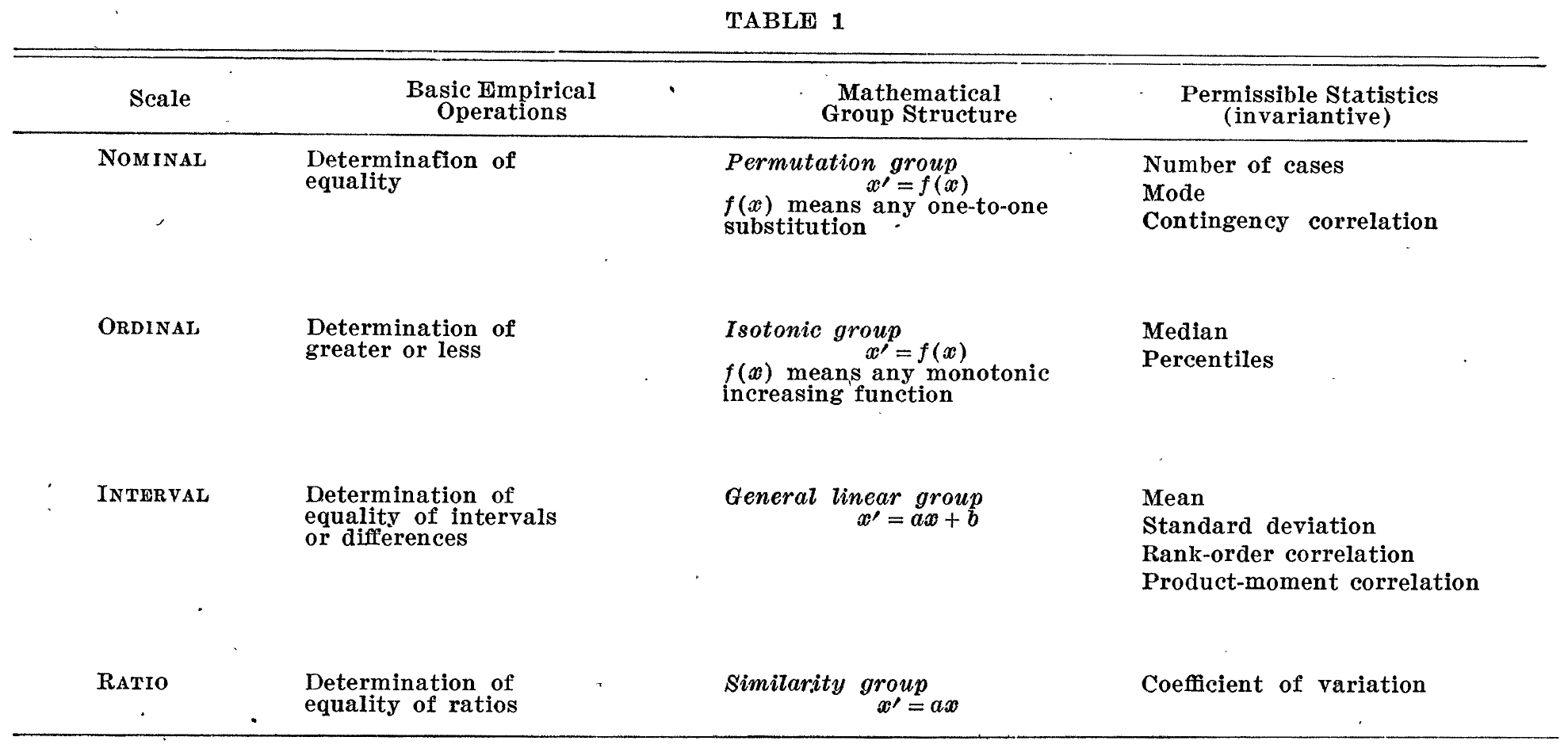
From S.S. Stevens, “On the Theory of Scales of Measurement (1946) Science. Volume 103, Number 2684.”
Stevens’ discussion on the analysis of ordinal data is very clear:
As a matter of fact, most of the scales used widely and effectively by psychologists are ordinal scales. In the strictest propriety the ordinary statistics involving means and standard deviations ought not to be used with these scales, for these statistics imply a knowledge of something more than the relative rank-order of data. On the other hand, for this ‘illegal’ statisticizing there can be invoked a kind of pragmatic sanction: In numerous instances it leads to fruitful results. While the outlawing of this procedure would probably serve no good purpose, it is proper to point out that means and standard deviations computed on an ordinal scale are in error to the extent that the sucessive intervals on the scale are unequal in size. When only the rank-order of the data is known, we should proceed cautiously with our statistics, and especially with the conclusions we draw from them.
Stevens’ discussion on the analysis of interval data:
Most psychological measurement aspires to create interval scales, and it sometimes succeeds. The problem usually is to devise operations for equalizing the units of the scales - a problem not always easy of solution but one for which there are several possible modes of attack. Only occaionally is there concern for the location of a ‘true’ zero point, because the human attributes measured by psychologists usually exist in a positive degree that is large compared with the range of its variation. In this respect these attributes are analogous to temerature as it is encountered in everyday life. Intelligence, for example, is usefully assessed on ordinal scales which try to approximate interval scales, and it is not necessary to define zero intelligence would mean.
Thus, although we assign numeric values to the responses, i.e., Strongly Approve (1), Approve (2), Undecided (3), Disapprove (4), and Strongly Dispprove (5), they can not be treated in the same manner as interval data, because they are ordinal in nature as described by Stevens. Consider the following questions:
- What is Strongly Disapprove minus Undecided?
- If we calculate \(5-3\), resulting in \(2\), how is the answer interpreted?
- Is it equal to Approve?
- What is Disapprove divided by Undecided?
- If we calculate \(4/3\) resulting in \(1.33\), how is the answer interpreted?
- Is it slightly less than Strongly Disapprove and Strongly Approve, respectively?
Clearly, we are assigning numerals to Likert responses to represent facts and conventions about the responses that are ranked (i.e. 1 is a more positive response/attitude than 5). The measurement of those numerals should directly relate to the type of scale (i.e., ordinal or interval). In the spirit of W.M. Kuzon Jr, M.G. Urbanchek, and S. McCabe (1996), the average of Strongly Approve and Approve is not Approve-and-a-half; regardless if we assign integers to represent Strongly Approve and Approve! Thus, in agreement with H.M. Marcus-Roberts and F.S. Roberts (1987), the answers to the Likert item with ordinal responses may have “meaningful statements”, but the basic empirical operations used to calculate means and standard deviations render “meaningless statistics.” Consider the following from P.A. Bishop and R.L. Herron (2015):
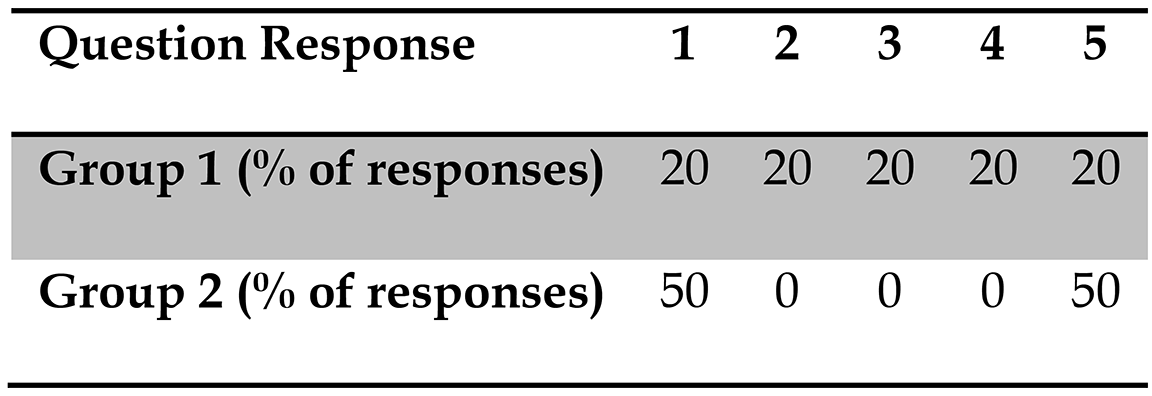
From P.A. Bishop and R.L. Herron (2015) “Use and Misuse of the Likert Item Responses and Other Ordinal Measures”, International Journal of Exercise Science, 8(3): 297-302. The authors discuss Clason and Dormoody’s (1994) critique of Likert response analysis- Regardless of the sample size, the means of the two groups would remain identical.
In practice, however, Likert scale response data are often treated as if it were interval data. In 1990, T.R. Knapp addressed the long standing controversy in depth, addressing key considerations on both the conservative (i.e., “pro-Stevens”) and liberal (i.e., “anti-Stevens”) sides. Basically the liberal practitioners argue that despite having strictly ordinal data, the differences between the responses are considered equal, and therefore treated at interval data. After all, B.O. Baker, C.D. Hardyk, and L.F. Petrinovich (1966), S. Labovitz (1967), G.V. Glass, P.D. Peckham and J.D. Sanders (1972) and others have shown empirically that doing so matters little (i.e., using parametric tests on ordinal data). Many modern day practitioners, such as J. Carifio and R. Perla (2008) and G. Norman (2010) continue to argue adamantly for the anti-Stevens position, in that violation of appropriateness is justified due to improvement in robustness. Certainly, as discussed by G.M. Sullivan and A.R. Artino (2013), improving the responses provided to begin with or implementing measurable visual analogue responses (VARs) helps to justify the use of parametric tests. Consider the following:
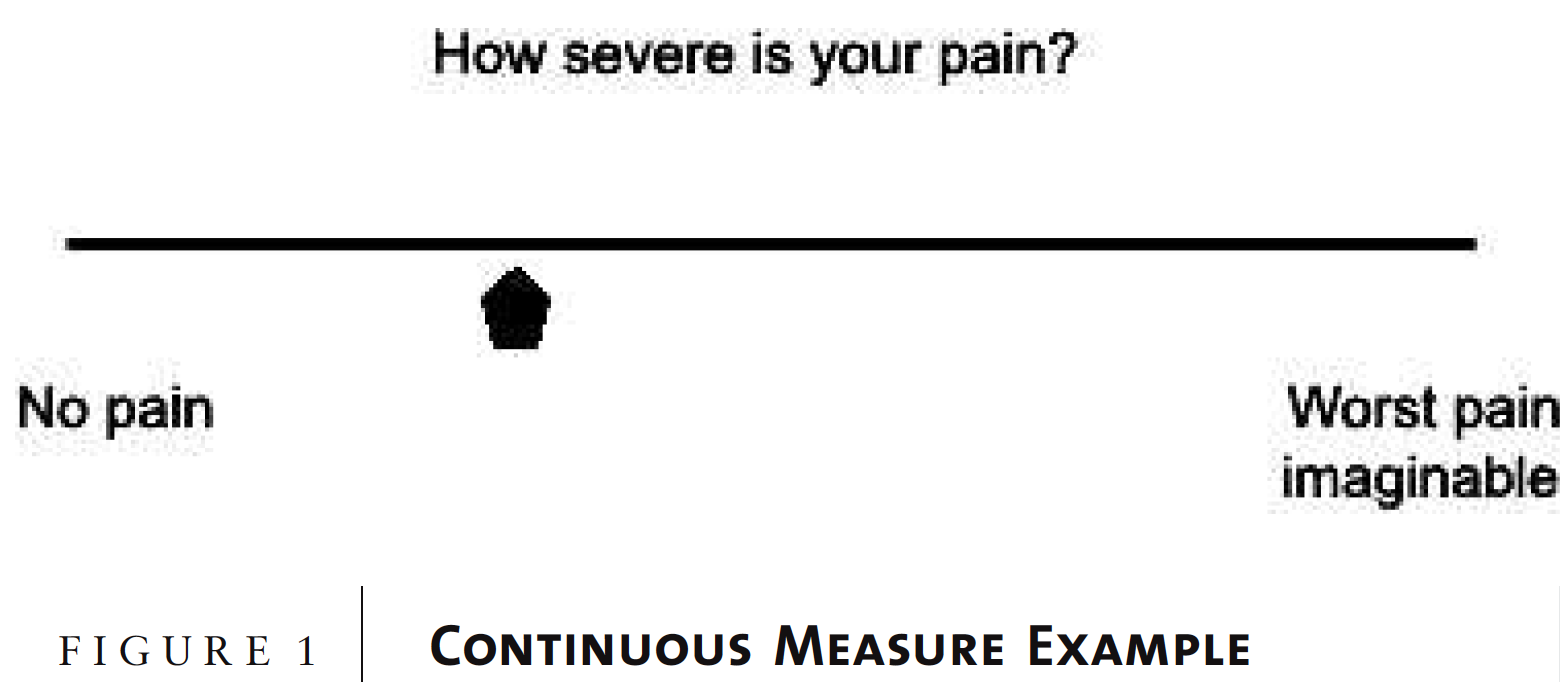
From G.M. Sullivan and A.R. Artino (2013) “Analyzing and Interpreting Data From Likert-Type Scales”, Journal of Graduate Medical Education, December, page 541. The visual analogue response can be physically measured 0-100 for interval data.
Knapp concludes, however, that “empirical robustness” are no longer convincing in light of H.M. Marcus-Roberts and F.S. Roberts (1987). Regardless of what side you decide to align with (conservative/pro-Stevens vs. liberal/anti-Stevens), Knapp ends his review with a set of guidelines:
Choose the measurement perspective. If the goal is to interpret the results in a scale-free manner, then follow the Stevens approach.
Practical concession to ‘illegal staticizing’ is OK when there are numerous data.
- When making up the scale and your goal is to have an interval scale, consider Stevens and ensure your scale reflects your intention.
- Is it continuous?
- Does it resemble an actual scale with units?
- Is there a zero value (even if arbitrary)?
- Do transformations preserve the order/meaningfulness?
Consider meaningfulness when considering the use of descriptive statistics. Knapp writes:
If you have to, forgo traditional statistics such as means, standard deviations, and Pearson r’s there are always Tukey’s (1977) very creative exploratory data analysis (EDA) techniques, and Agresti (1984) has written a whole book on the analysis of ordinal data.
In 2001, A. Agresti published a fantastic book on “Categorical Data Analysis.” You also may consider Hoaglin, Moesttler and J.W. Tukey (2001) “Understanding Robust and Exploratory Data Analysis” instead.
- The type of scale of data claimed will determine the use of non-parametric or parametric tests.
In conclusion, I recommend taking time to familiarize yourself with Steven and Knapp. Ultimately, you have to decide how you want to analyze the data. Below, I provide code to visualize likert data, and conduct both non-paramteric and parametric analyses.
Basic Likert Data Analysis
Dataset
To demonstrate the Likert analysis workflow, I’ll use the MACH-IV dataset, which is a freely available download. It draws on answers from Christie, R. & Geis, F. (1970) “Studies in Machiavellianism”. NY: Academic Press.), which is a tool that is used to measure Machiavellianism personality traits. The test consists of twenty Likert items. Each item is a statement that you must indicate how accurate it would be when applied to you. The data are presented in wide form with each row as a single observation.
- Answers: 1 = strongly disagree, 2 = disagree, 3 = neutral, 4 = agree, 5 = strongly agree (0 = they skipped). For the puposes of this analysis, we will consider the responses to be ordinal.
- Age: Entered into a text field.
- Gender: Chosen from a drop down list (1 = male, 2 = female, 3 = other; 0 = no answer)
- Questions:
- Q1. Never tell anyone the real reason you did something unless it is useful to do so.
- Q2. The best way to handle people is to tell them what they want to hear.
- Q3. One should take action only when sure it is morally right.
- Q4. Most people are basically good and kind.
- Q5. It is safest to assume that all people have a vicious streak and it will come out when they are given a chance.
- Q6. Honesty is the best policy in all cases.
- Q7. There is no excuse for lying to someone else.
- Q8. Generally speaking, people won’t work hard unless they’re forced to do so.
- Q9. All in all, it is better to be humble and honest than to be important and dishonest.
- Q10. When you ask someone to do something for you, it is best to give the real reasons for wanting it rather than giving reasons which carry more weight.
- Q11. Most people who get ahead in the world lead clean, moral lives.
- Q12. Anyone who completely trusts anyone else is asking for trouble.
- Q13. The biggest difference between most criminals and other people is that the criminals are stupid enough to get caught.
- Q14. Most people are brave.
- Q15. It is wise to flatter important people.
- Q16. It is possible to be good in all respects.
- Q17. P.T. Barnum was wrong when he said that there’s a sucker born every minute.
- Q18. It is hard to get ahead without cutting corners here and there.
- Q19. People suffering from incurable diseases should have the choice of being put painlessly to death.
- Q20. Most people forget more easily the death of their parents than the loss of their property.
Perhaps our research question will be to determine whether men and women demonstrate a signficant difference in Machiavellianism personality traits. We will examine each question individually, and then evaluate total score, treating that measure as interval data. Let’s start by downloading the dataset:
url <- "http://personality-testing.info/_rawdata/MACH2.zip"  # web address of dataset

if (!file.exists("./MACH2.zip")) {
    download(url, dest = "MACH2.zip", mode = "wb")  # download zip file
    unzip("MACH2.zip", exdir = "./")  # unzip datafiles into a folder /MACH2
}

ds <- "/MACH2/data.csv"  # the data set of interest
cb <- "/MACH2/codebook.txt"  # the code to the questions

dt <- data.frame(read_csv(paste(wd, ds, sep = "")))  # import data into a data.table

dtQ <- data.table(read_lines(paste(wd, cb, sep = ""))[3:22])  # reading the lines of the questions from the text file

dtQ[, `:=`(c("question", "question_text"), tstrsplit(V1, "[0-9]. ", fixed = TRUE))]  # splits the 'QX. from the Questions.' at the first '.' after a digit.

colnames(dt)[1:20] <- dtQ$question_text[1:20]  # colnames to full questions

posQ <- colnames(dt)[c(1:2, 5, 8, 12:13, 15, 17:20)]  # postive questions
negQ <- colnames(dt)[c(3:4, 6:7, 9:11, 14, 16)]  # negative questions
Explore data and remove outliers
Before we begin the analysis, let’s explore the data and remove outliers in the demographic and total score columns. The scores reflect a minimum of \(20\) and maximum of \(100\) points. When we assign gender as a factor with two levels (male and female), those respondents that did not answer will be removed when we remove NAs. Obviously there are issues with age, with a range of -9 to 999999. We will limit the respondents from 10 to 100 years old. In a similar manner, the range for elapsed time is very large. We will limit seconds_elapsed from 60 seconds (3 seconds per question) to 600 (30 seconds per question). Finally, once we limit respondents to those who answered every question, create factors and levels for each question, most of the outlier questions will be removed.
First, let’s take a look at gender first:
Number of Respondents By Gender
dt[, 1:20] <- lapply(dt[, 1:20], factor, levels = c(1, 2, 3, 4, 5), labels = c("strongly disagree",
    "disagree", "neutral", "agree", "strongly agree"))  # change columns to factors

dt$gender <- factor(dt$gender, levels = c(1, 2), labels = c("male", "female"))  # change to factor

plot_ly(data = as.data.frame(dt), x = ~gender)
There are quite a few more male respondents than female. Now let’s take a look at age:
Distribution of Age
dt <- dt[dt$age < 110 & dt$age >= 10, ]  # remove observatons with ages outside of 18 - 100.

dt <- na.omit(dt)  # remove respondents with NAs

plot_ly(data = as.data.frame(dt), x = ~age)  # histogram of age
Most of the respondents are fairly young. Next, lets take a look at seconds_elapsed:
Distrubtion of Seconds Elapsed
dt <- dt[dt$seconds_elapsed < 1200 & dt$seconds_elapsed >= 60, ]  # remove observatons outside of 60 - 1200 seconds.

plot_ly(data = as.data.frame(dt), x = ~seconds_elapsed)  # histogram of seconds_elapsed
The vast majority of repondents spend very less than 4 minutes on then questionnaire. Finally, let’s take a look at the distribution of scores:
Distrubtion of Scores (Machiavellianism Index)
plot_ly(data = as.data.frame(dt), x = ~score) # histogram of ageThe total scores are normally distributed. The scores are a composite of all the answers. The range is 20-100. The test
pt <- tabular(gender ~ (age + seconds_elapsed + score) * (mean + sd), data = dt)

pander(pt)
gender |
age mean |
sd |
seconds_elapsed mean |
sd |
score mean |
sd |
|---|---|---|---|---|---|---|
| male | 28.72 | 11.59 | 238.5 | 155.7 | 67.89 | 13.03 |
| female | 29.88 | 12.17 | 255.1 | 175.1 | 62.51 | 12.41 |
Descriptive Statistics
According to Stevens, descriptive statistics for ordinal data should be median. But first, one simple method to visualize the percentages by gender is to use the likert function in the likert package. These figures allow you to group by a factor, and provides color coordinated horizontal bar charts to compare the percent of answers.
dt_pos <- dt[posQ]  # select only the 11 positive questions according to the codetext

dt_pos$gender <- dt$gender  # create a standalone data.table for this analysis.

mach_l1 <- likert::likert(dt_pos[, 1:4, drop = FALSE], grouping = dt_pos$gender)  # view the first 4 (1:4 questions) and group them by gender
likert.bar.plot(mach_l1)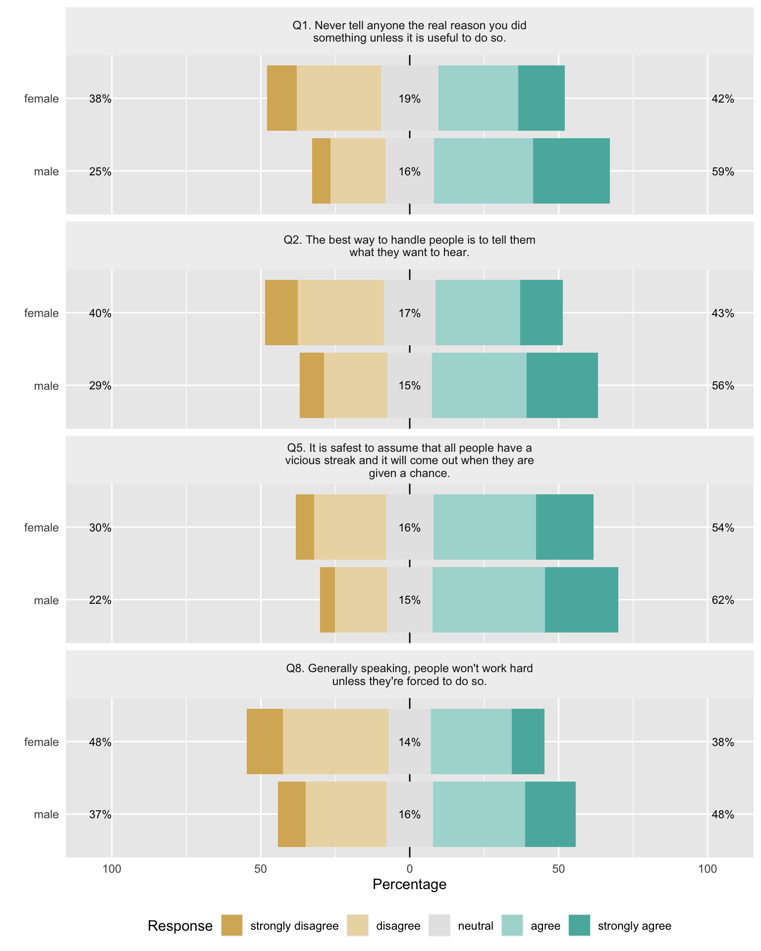
Similarly, you can look at the fiirst 4 negative questions. These visual graphics take up quite a bit of room.
dt_neg <- dt[negQ]
dt_neg$gender <- dt$gender
mach_l2 <- likert::likert(dt_neg[, 1:4, drop = FALSE], grouping = dt_neg$gender)
likert.bar.plot(mach_l2)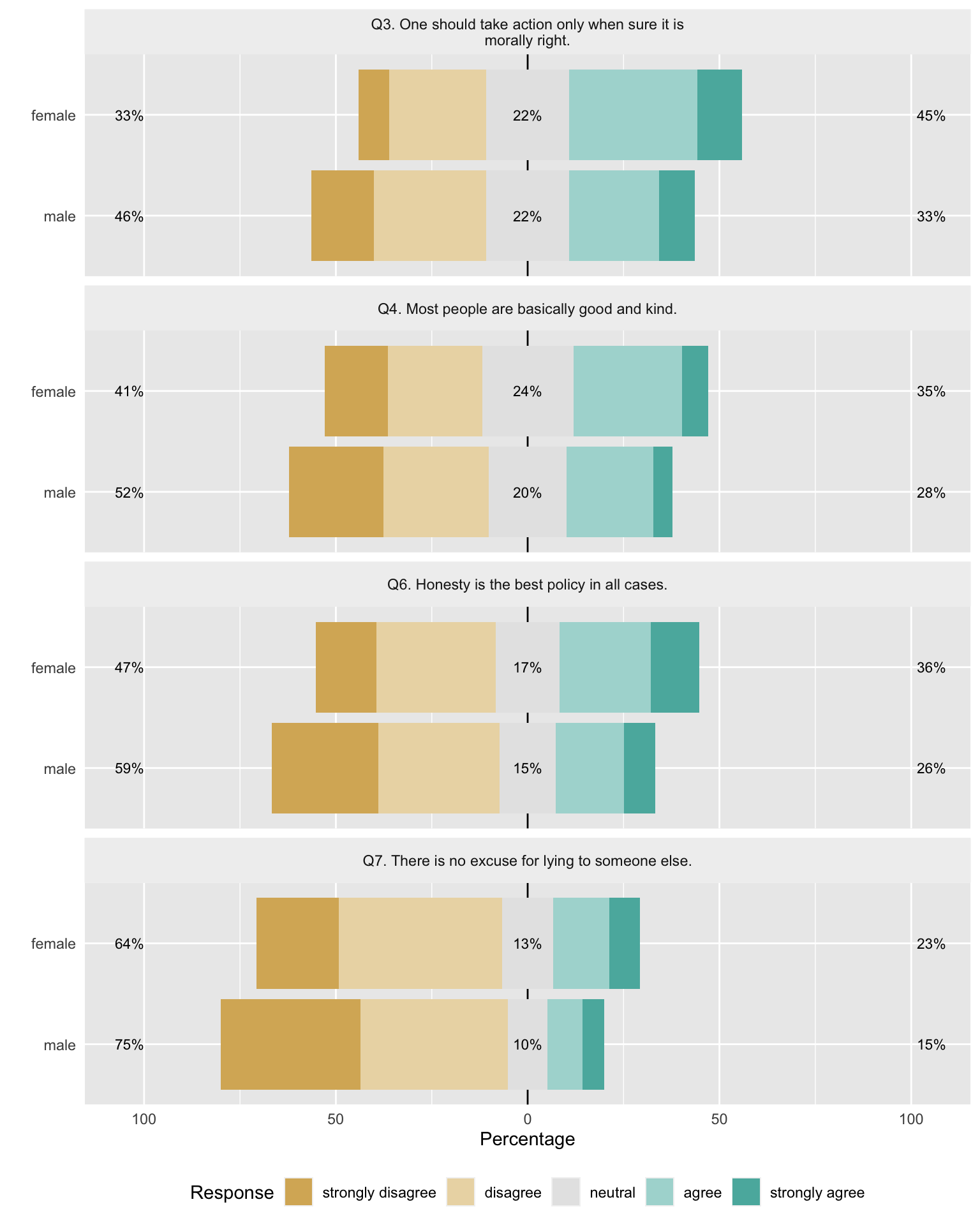
In the following examples, I’ve selected the first 2 questions from males to show the summary tables that sjtPlot provides with the sjt.frq function.
library(arsenal)
# Controls used for the arsenal package / demographics tables
mycontrols <- tableby.control(test = TRUE, total = TRUE, digits = 1, numeric.test = "anova",
    cat.test = "chisq", ordered.test = "trend", numeric.stats = c("N", "meansd",
        "medianrange", "q1q3", "iqr"), cat.stats = c("countpct"), stats.labels = list(N = "Number",
        meansd = "Mean (SD)", medianrange = "Median (Range)", q1q3 = "Q1, Q3", iqr = "IQR"))

dtt <- dt
colnames(dtt)[c(1:20, 22)] <- c("Q1", "Q2", "Q3", "Q4", "Q5", "Q6", "Q7", "Q8", "Q9",
    "Q10", "Q11", "Q12", "Q13", "Q14", "Q15", "Q16", "Q17", "Q18", "Q19", "Q20",
    "Sex")
tab1 <- tableby(Sex ~ Q1 + Q2, data = dtt, control = mycontrols)
t1 <- "Q1 = Never tell anyone the real reason you did something unless it is useful to do so. Q2 = The best way to handle people is to tell them what they want to hear. N = Number, Q1 = First Quartile, Q3 = Third Quartile, SD = Standard Deviation."
summary(tab1, text = F, pfootnote = T, title = t1)| male (N=7692) | female (N=4079) | Total (N=11771) | p value | |
|---|---|---|---|---|
| Q1 | < 0.0011 | |||
| strongly disagree | 483 (6.3%) | 409 (10.0%) | 892 (7.6%) | |
| disagree | 1419 (18.4%) | 1148 (28.1%) | 2567 (21.8%) | |
| neutral | 1245 (16.2%) | 792 (19.4%) | 2037 (17.3%) | |
| agree | 2564 (33.3%) | 1089 (26.7%) | 3653 (31.0%) | |
| strongly agree | 1981 (25.8%) | 641 (15.7%) | 2622 (22.3%) | |
| Q2 | < 0.0011 | |||
| strongly disagree | 622 (8.1%) | 450 (11.0%) | 1072 (9.1%) | |
| disagree | 1637 (21.3%) | 1177 (28.9%) | 2814 (23.9%) | |
| neutral | 1153 (15.0%) | 709 (17.4%) | 1862 (15.8%) | |
| agree | 2445 (31.8%) | 1158 (28.4%) | 3603 (30.6%) | |
| strongly agree | 1835 (23.9%) | 585 (14.3%) | 2420 (20.6%) |
- Pearson’s Chi-squared test
rm(tab1, td1, t1)

# sjt.frq(dt[dt$gender == 'male',c(1:2)], emph.md = TRUE, show.summary = FALSE,
# emph.quart = TRUE, no.output = FALSE) # the sjtPlot provides quite a few
# options! emph.md emphasizes the median, emph.quart draws a line are the
# quartiles.  If you show.summary = TRUE, it provides mean, sigma and other
# values in the bottom of the table.
sjt.grpmean(var.cnt = score, var.grp = gender, digits = 1, no.output = FALSE)## Error in sjt.grpmean(var.cnt = score, var.grp = gender, digits = 1, no.output = FALSE): could not find function "sjt.grpmean"Statistical Inference Techniques
The Wilcoxon tests is performed in R with the wilcox.test function, which uses binary factors, such as Gender (M/F), or Pre-Post Analysis. For example, if only Pre-scores are given, or if both Pre-scores (\(x\)) and Post-Scores (\(y\)) are given and paired is TRUE (i.e., the same person’s answers), a Wilcoxon signed rank test of the null that the distribution of \(x\) (in the one sample case) or of \(x\) - \(y\) (in the paired two sample case) is symmetric about \(\mu\) is performed. Our example analysis will use gender and a single likert question.
library(FSA)
dt_wc <- dt

dt_wc$`Q1. Never tell anyone the real reason you did something unless it is useful to do so.` <- as.numeric(dt_wc$`Q1. Never tell anyone the real reason you did something unless it is useful to do so.`)

kable(Summarize(`Q1. Never tell anyone the real reason you did something unless it is useful to do so.` ~
    gender, data = dt_wc, digit = 3)) %>% kable_styling(bootstrap_options = "basic",
full_width = F)| gender | n | mean | sd | min | Q1 | median | Q3 | max |
|---|---|---|---|---|---|---|---|---|
| male | 7692 | 3.538 | 1.229 | 1 | 3 | 4 | 5 | 5 |
| female | 4079 | 3.099 | 1.252 | 1 | 2 | 3 | 4 | 5 |
wt <- wilcox.test(as.numeric(dt_wc[, 1]) ~ as.factor(gender), data = dt_wc, alternative = "two.sided",
    exact = FALSE)

print(wt)
Wilcoxon rank sum test with continuity correction
data: as.numeric(dt_wc[, 1]) by as.factor(gender) W = 18789658, p-value < 2.2e-16 alternative hypothesis: true location shift is not equal to 0
The Kruskal Wallis test is performed in R with the kruskal.test function, which uses multivariate factors, such as Education & Certification Levels (Associates, Bachelors, Masters, or Doctorates. The current study does not contain multivariate data. I randomly added unknown gender to the categories, such that it is now multivariate.
dt_kw <- dt

dt_kw$gender <- factor(dt_kw$gender, levels = c("male", "female", "unknown"))  # create a third category
dt_kw$gender[sample(nrow(dt_kw), 2000)] <- "unknown"  # label

dt_kw$`Q1. Never tell anyone the real reason you did something unless it is useful to do so.` <- as.numeric(dt_kw$`Q1. Never tell anyone the real reason you did something unless it is useful to do so.`)

kable(Summarize(`Q1. Never tell anyone the real reason you did something unless it is useful to do so.` ~
    gender, data = dt_kw, digit = 3)) %>% kable_styling(bootstrap_options = "basic",
full_width = F)| gender | n | mean | sd | min | Q1 | median | Q3 | max |
|---|---|---|---|---|---|---|---|---|
| male | 6373 | 3.539 | 1.229 | 1 | 3 | 4 | 5 | 5 |
| female | 3398 | 3.104 | 1.244 | 1 | 2 | 3 | 4 | 5 |
| unknown | 2000 | 3.378 | 1.269 | 1 | 2 | 4 | 4 | 5 |
kt <- kruskal.test(as.numeric(dt_kw[, 1]) ~ as.factor(gender), data = dt_kw)

print(kt)
Kruskal-Wallis rank sum test
data: as.numeric(dt_kw[, 1]) by as.factor(gender) Kruskal-Wallis chi-squared = 272.66, df = 2, p-value < 2.2e-16
The One-Way ANOVA is a multivariate analysis only used when ordinal data (Likert data) are transformed to interval data. The data, however, still have to meet the assumptions of the test (normality, etc.). For example, the ordinal data can be ordered, and then a table is produced and the data converted to probability or frequency. For this analysis we used the score values and
For the interval data, such as scores, we can use the HH packages to conduct an ANOVA. The hov and hovPlot functions indicate:
Oneway analysis of variance makes the assumption that the variances of the groups are equal. Brown and Forsyth, 1974 present the recommended test of this assumption. The Brown and Forsyth test statistic is the F statistic resulting from an ordinary one-way analysis of variance on the absolute deviations from the median.
The “trellis” object with three panels containing boxplots for each group: The observed data “y”, the data with the median subtracted “y-med(y)”, and the absolute deviations from the median “abs(y-med(y))” The Brown and Forsyth test statistic is the F statistic resulting from an ordinary one-way analysis of variance on the data points in the third panel.
library(HH)

dt_gen <- dt

dt_gen$gender <- factor(dt_gen$gender, levels = c("male", "female", "unknown"))  # create a third category
dt_gen$gender[sample(nrow(dt_gen), 2000)] <- "unknown"  # label

hovPlot(as.numeric(score) ~ as.factor(gender), data = dt_gen)  # example test of the assumtions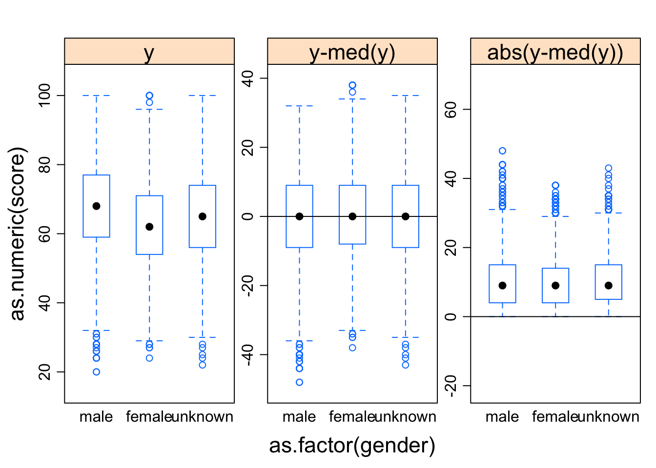
library(texreg)
hv <- hov(as.numeric(score) ~ as.factor(gender), data = dt_gen)  # example parametric test
hv <- hov(as.numeric(score) ~ as.factor(gender), data = dt)
screenreg(hv)
## Error in (function (classes, fdef, mtable) : unable to find an inherited method for function 'extract' for signature '"htest"'set.seed(101)
fac_num <- function(x) {
if (x == "strongly disagree") {
x = 1
}
if (x == "disagree") {
x = 2
}
if (x == "neutral") {
x = 3
}
if (x == "agree") {
x = 4
}
if (x == "strongly agree") {
x = 5
}
}
dt_gen_num <- sapply(dt_gen[, c(1:20)], function(x) as.integer(factor(as.character(x),
levels = c("strongly disagree", "disagree", "neutral", "agree", "strongly agree"))))
dt_gen_num <- cbind(dt_gen_num, dt_gen[, c(21:24)])
colnames(dt_gen_num) <- colnames(dt_gen)
mat <- dt_gen_num[, c(1:20)]
myPCA <- prcomp(mat, scale. = F, center = F)
plot(myPCA)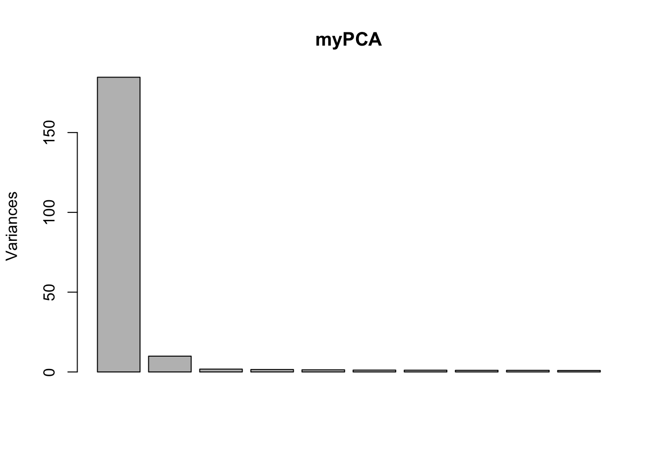
# myPCA$rotation # loadings myPCA$x # scores
biplot(myPCA, scale = 0)
# Perform SVD
mySVD <- svd(mat)
# mySVD # the diagonal of Sigma mySVD$d is given as a vector
sigma <- matrix(0, 20, 20)  # we have 4 PCs, no need for a 5th column
diag(sigma) <- mySVD$d  # sigma is now our true sigma matrix


# Compare PCA scores with the SVD's U*Sigma
theoreticalScores <- mySVD$u %*% sigma
all(round(myPCA$x, 5) == round(theoreticalScores, 5))  # TRUE
[1] TRUE
# Compare PCA loadings with the SVD's V
all(round(myPCA$rotation, 5) == round(mySVD$v, 5))  # TRUE
[1] TRUE
# Show that mat == U*Sigma*t(V)
recoverMatSVD <- theoreticalScores %*% t(mySVD$v)
all(round(mat, 5) == round(recoverMatSVD, 5))  # TRUE
[1] TRUE
# Show that mat == scores*t(loadings)
recoverMatPCA <- myPCA$x %*% t(myPCA$rotation)
all(round(mat, 5) == round(recoverMatPCA, 5))  # TRUE
[1] TRUE
plot(myPCA$x)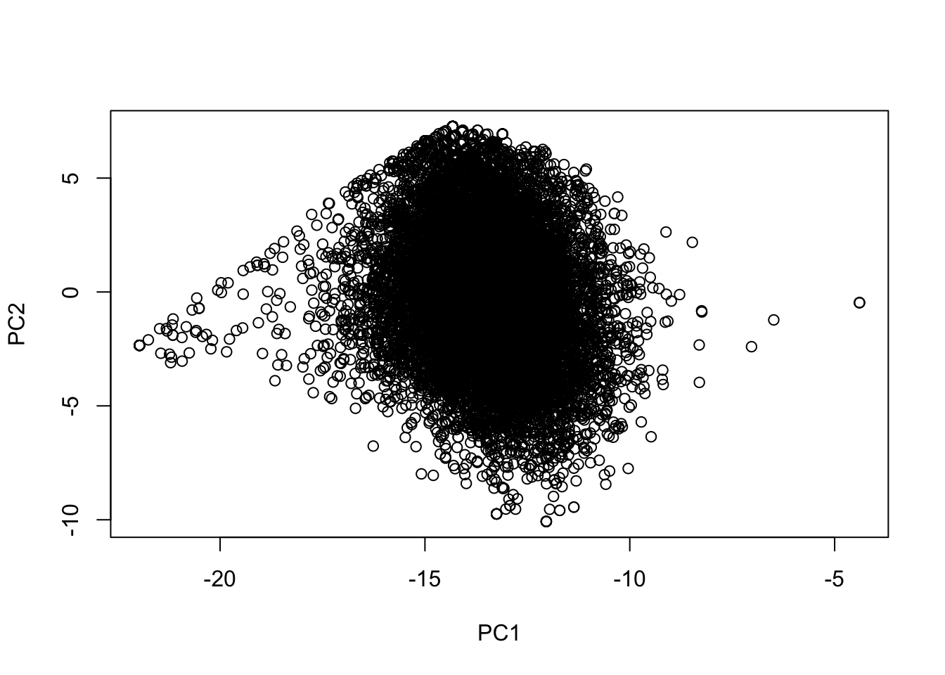
library(survey)Finally, regression techniques include Ordered logistic regression, Multinomial logistic regression, or we could collapse the levels of the Dependent variable into two levels and run binary logistic regression. Regression models are ways to develop predictive models based on the questions.
Until next time…
